Soft Sensors for Energy Consumption in Topographic Uncertainty Propagation
June 1, 2026
Introduction
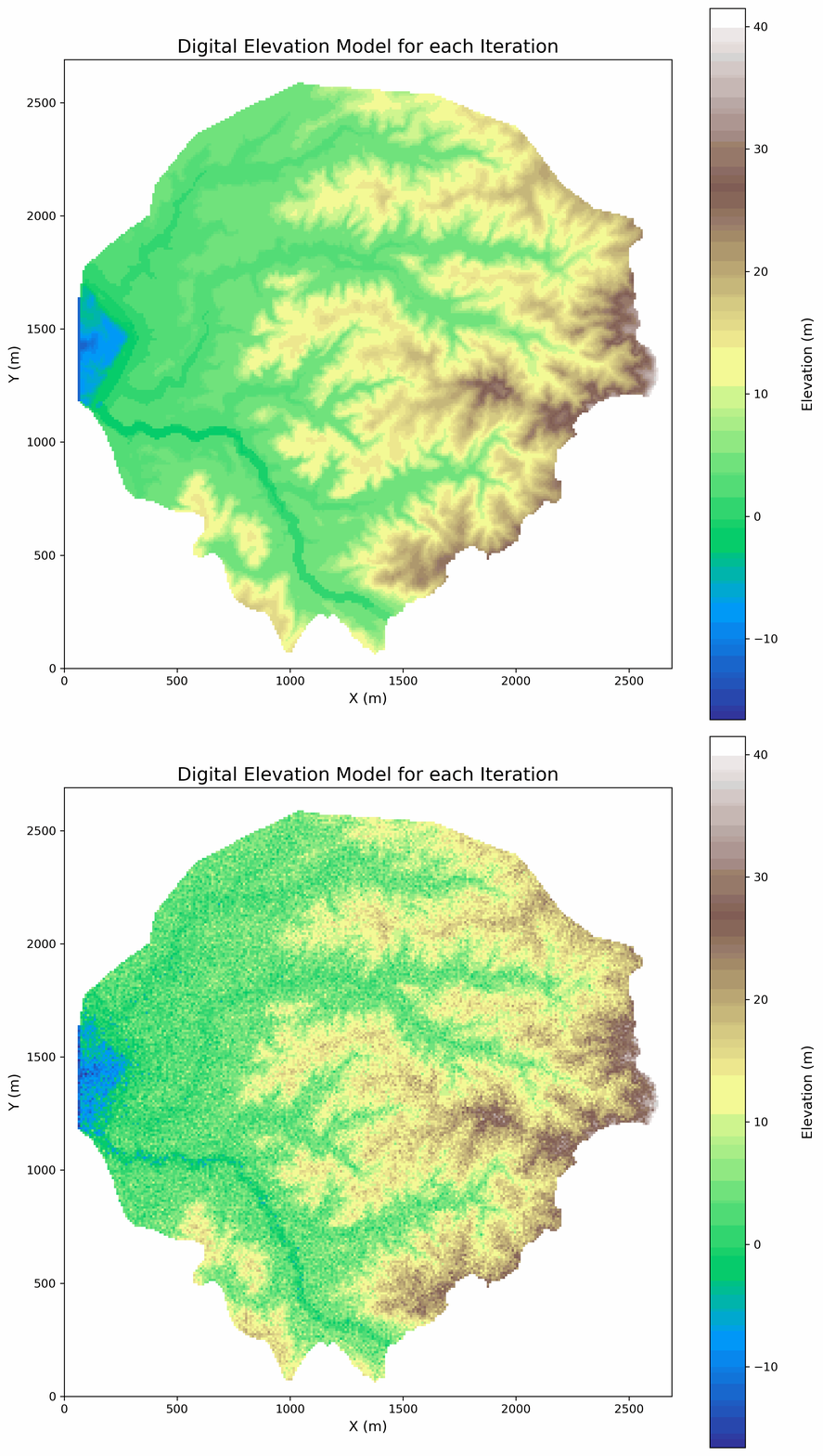
Figure 1: Original vs. Noisy DEM
The Impact of DEM Uncertainty
“Overlooking DEM uncertainty may lead to a bias in risk management decisions” [1]
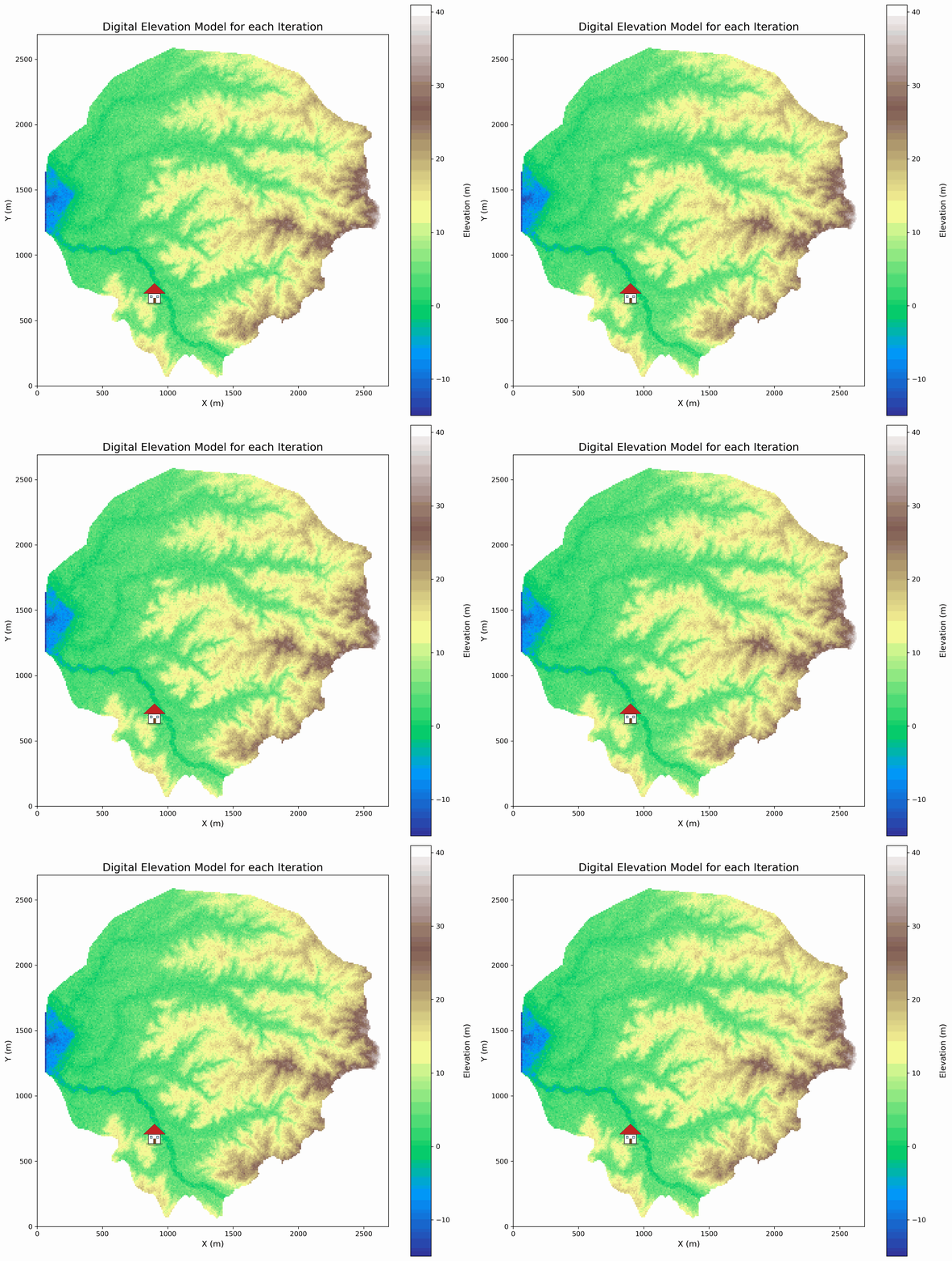
The Impact of DEM Uncertainty
Quantity of Interest: Water depth at the houses coordinates
| \(\sigma_{input}\) (m) | Mean (m) | Std. Dev (m) | CV (%) |
|---|---|---|---|
| 0.05 | 0.739 | \(\pm 0.050\) | 6.78% |
| 0.1 | 0.756 | \(\pm 0.110\) | 14.50% |
| 0.2 | 0.774 | \(\pm 0.206\) | 26.61% |
| 0.5 | 0.880 | \(\pm 0.446\) | 50.71% |
| 1.0 | 1.101 | \(\pm 0.817\) | 74.21% |
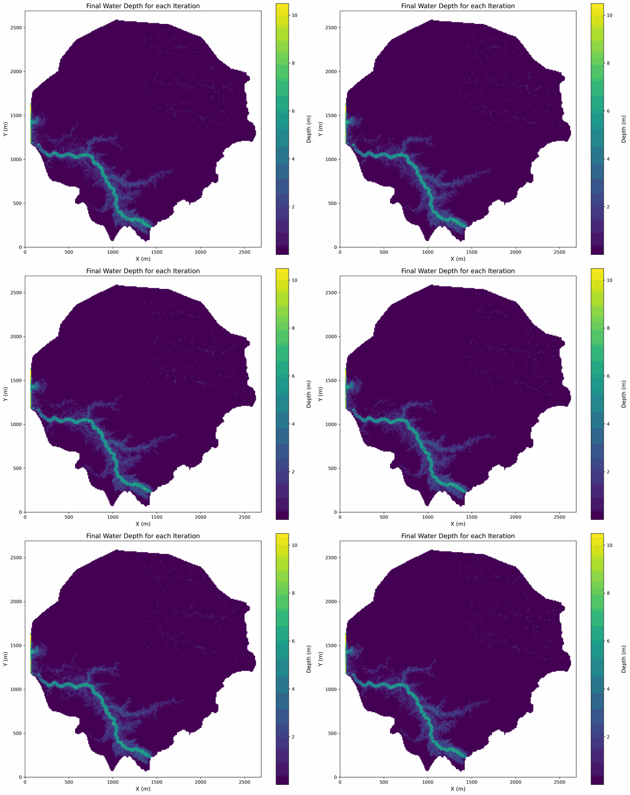
Figure 3: Water depth uncertainty propagation.
Is Execution Time a Reliable Proxy?
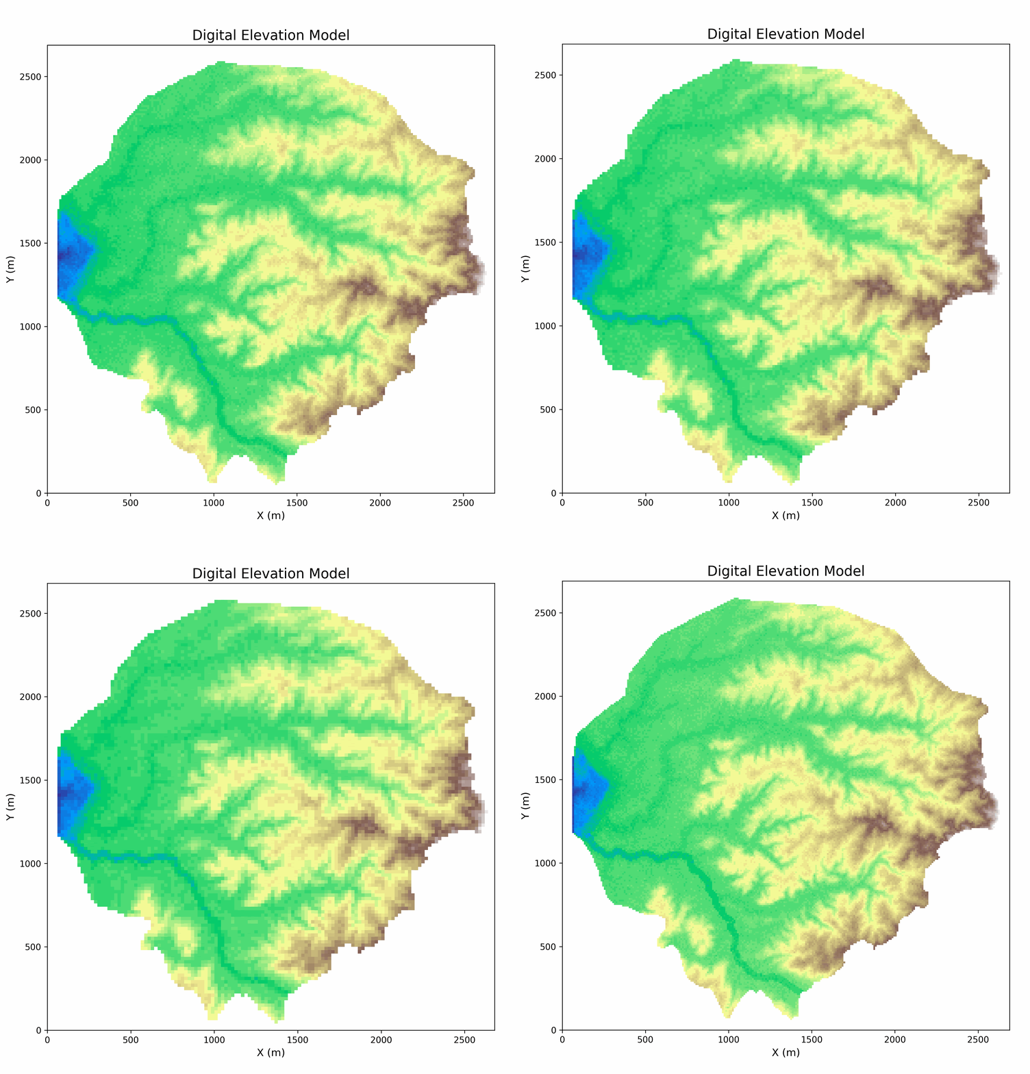
Figure 5: Comparison of Original and Downsampled DEM Resolutions
Is Execution Time a Reliable Proxy?
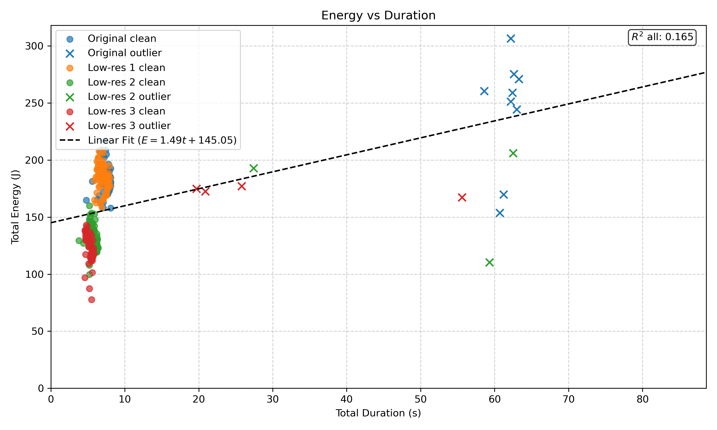
Figure 6: Total energy consumption vs. execution duration for all iterations
Is Execution Time a Reliable Proxy?
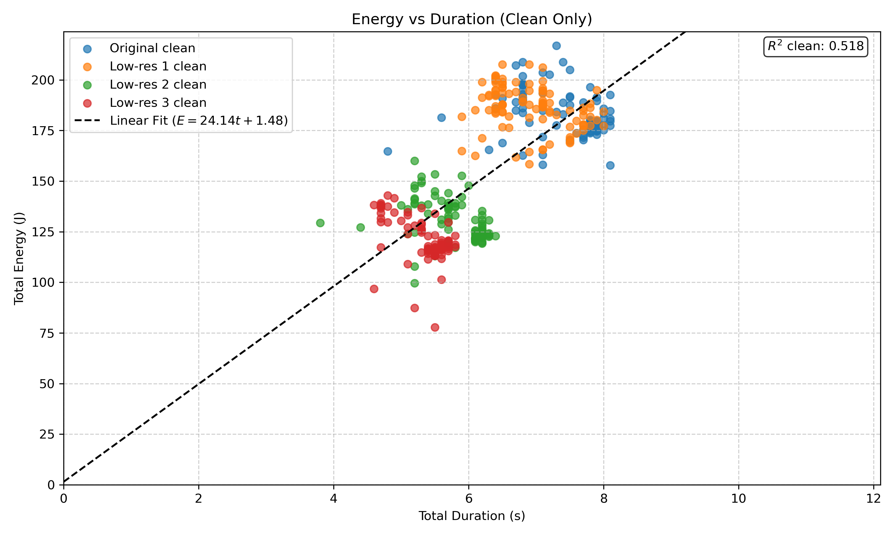
Figure 7: Total energy consumption vs. execution duration for all clean iterations
Is Execution Time a Reliable Proxy?
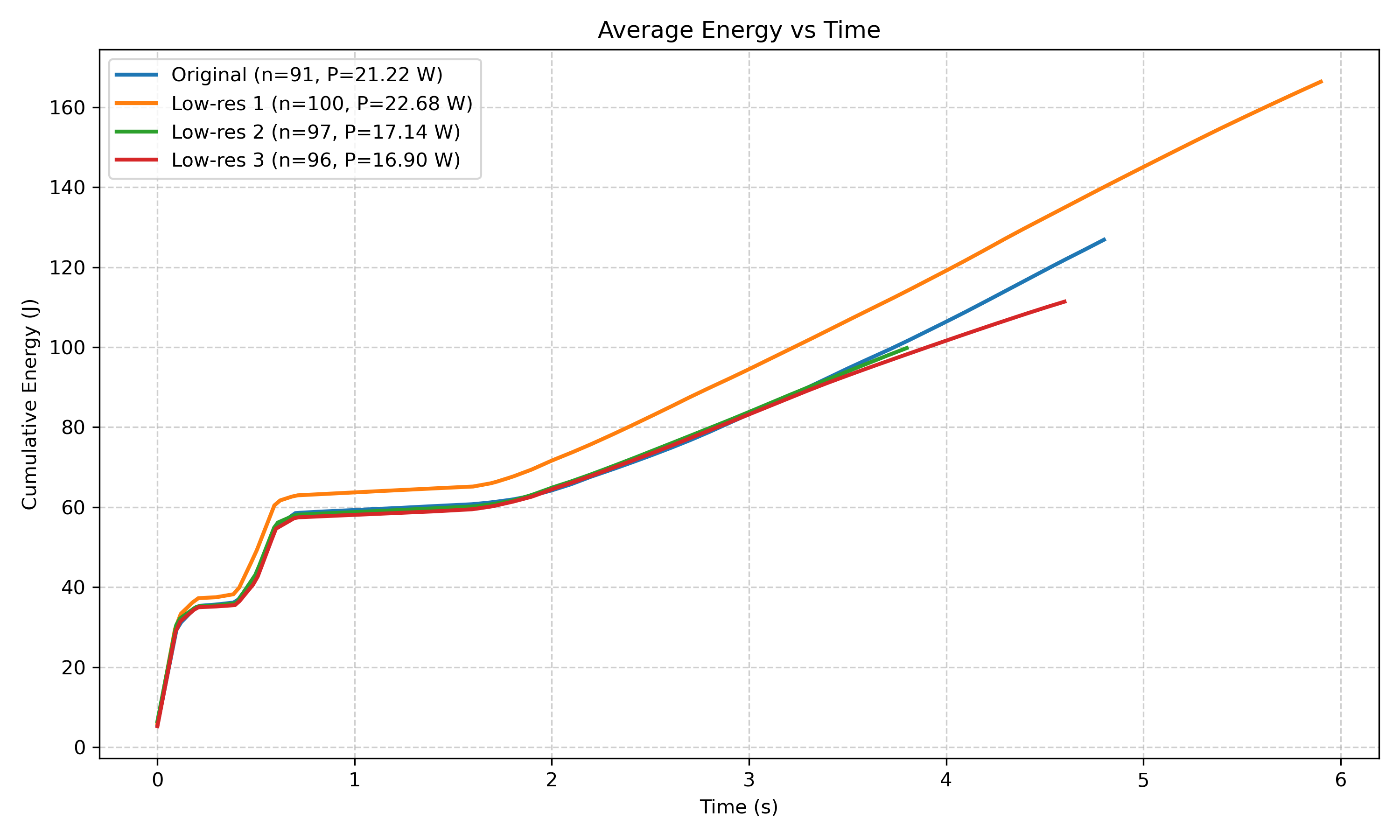
Figure 8: Average Cumulative Energy-Time Plot
Uncertainty Quantification in consumed Energy
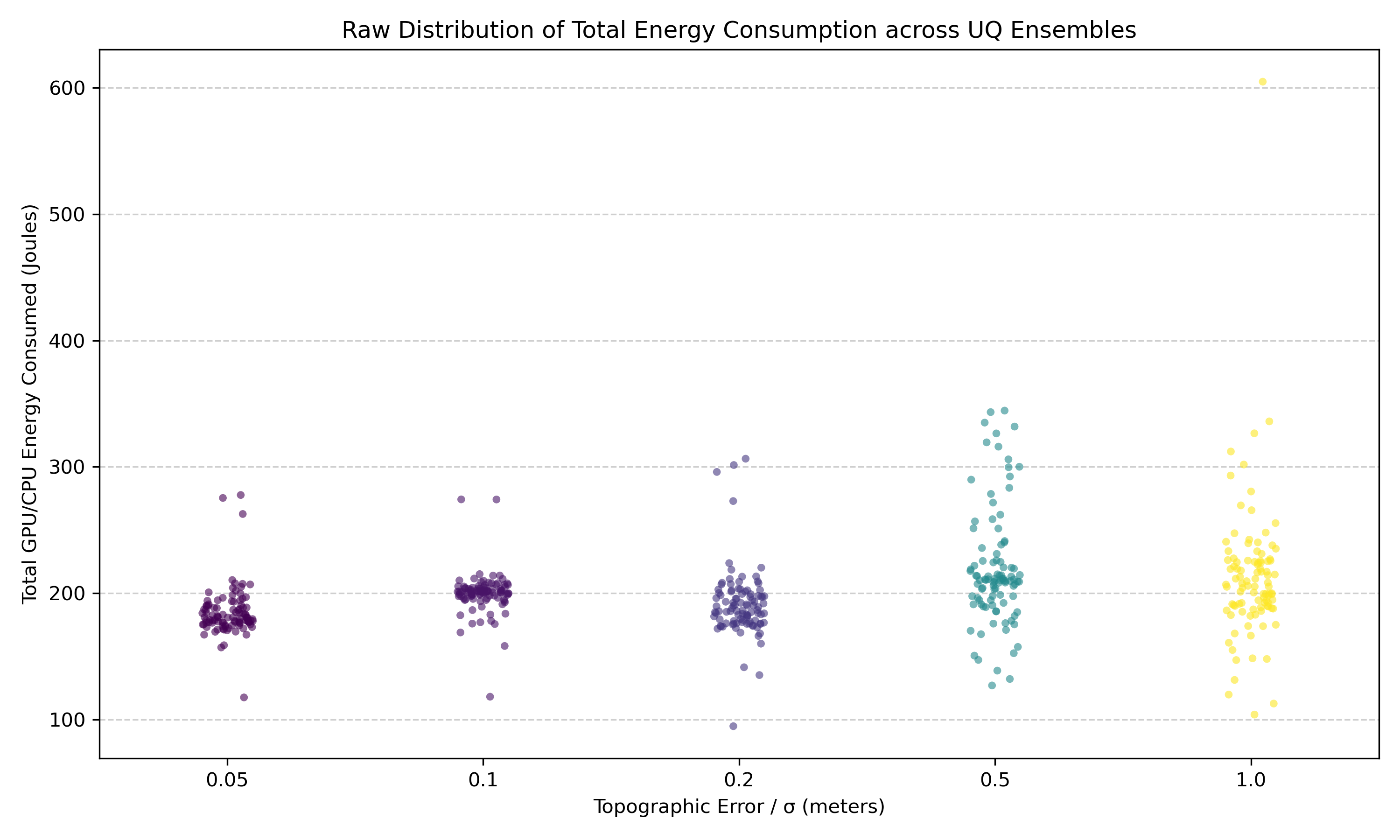
Figure 9: Raw distribution of total energy consumption for each topographic noise level
Uncertainty Quantification in consumed Energy
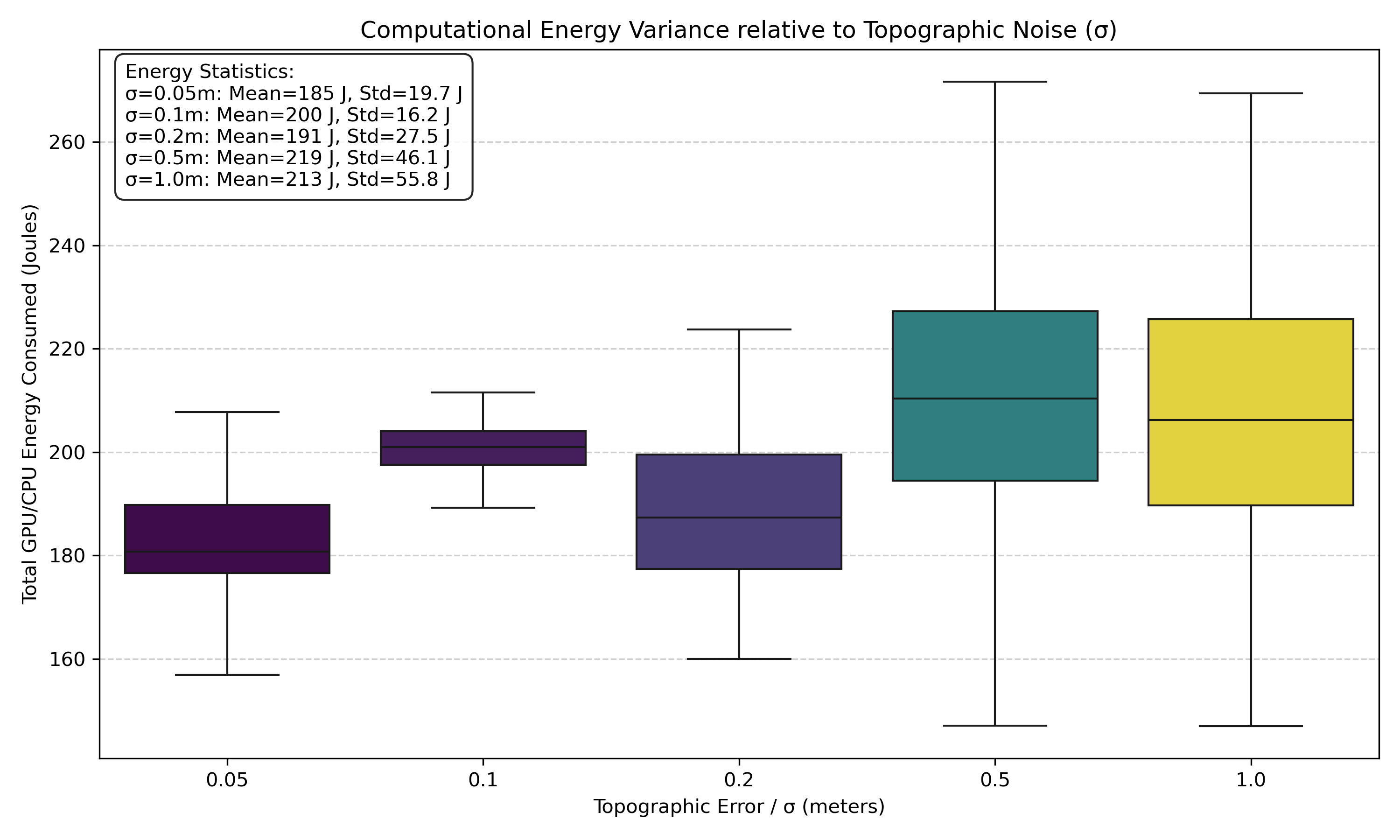
Figure 10: Statistical distribution of total energy consumption for each topographic noise level